The Quest for the Perfect Nav Log (Part 1 - E6B Computations)

After putting together the early versions of my VFR navigation log and developing its IFR counterpart, I became interested in automating more and more of the process of putting together a fully featured navigation log. In this series of posts, I will cover ways to automate navigation, performance, aircraft information, and finally building a front-end for the nav log builder.

In this first part, we’ll start easy, and we’ll look at how we can use Google Sheets to help us run some of the E6B computations.

Automated E6B computations

Google Sheets and Excel have a full range of trigonometry functions which make it easy to compute wind correction angles and ground speed values.

This first level of automation still has you go on your sectional to find true courses, leg distances, and requires true airspeed, fuel consumption, and wind aloft information from your performance and weather planning. We’ll look at automating these later in this article and the series.

Wind correction angle

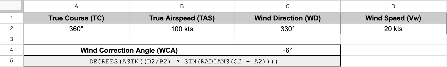
With the following cell assignment:

• True Course (TC) in cell A2
• True Airspeed (TAS) in cell B2
• Wind Direction (WD) in cell C2
• Wind Speed (Vw) in cell D2

The following formula yields the wind correction angle:

=DEGREES(ASIN((D2/B2) * SIN(RADIANS(C2 - A2))))

You can see an example below, and look at an example worksheet here. Feel free to make a copy and play with it.

Groundspeed

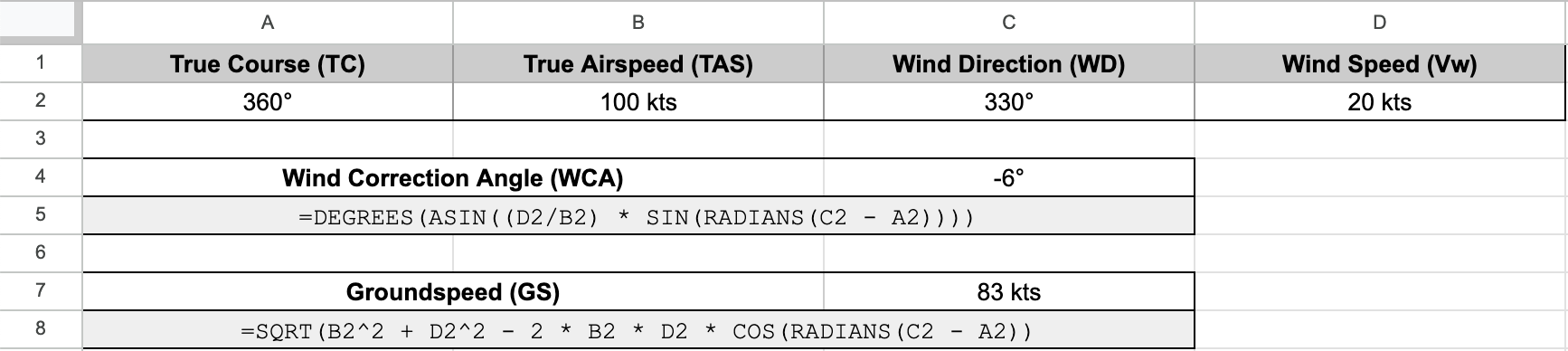
With the same cell assignment as above, the following formula yields the groundspeed:

=SQRT(B2^2 + D2^2 - 2 * B2 * D2 * COS(RADIANS(C2 - A2))

Look at the worksheet above to see it live!

Estimated time enroute

Now that we have our groundspeed number, using our the leg distance we measured, we are able to derive our Estimated time enroute. Time is distance divided by speed, but where it can get confusing is how Google Sheets handles time. You must have all your durations entered as a fraction of a day. For example, 3 hours is 3/24 = 0.125 days. From that value, Google Sheets is able to format your duration in a variety of ways, including the familiar hh:mm (e.g. 03:24 for 3 hours 24 minutes) format, or mm:ss (e.g 03:45 for 3 minutes 45 seconds). If your durations are not entered as fraction of a day, none of the formatting and computing will work.

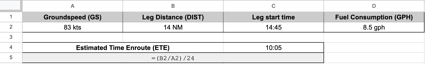
With the following cell assignment:

• Groundspeed (GS) in cell A2
• Leg Distance (DIST) in cell B2

The following formula yields the estimated time enroute:

=(B2/A2)/24

You can see an example below, and look at the second tab in the example worksheet here.

Estimated time of arrival

Computing our estimated time of arrival is a simple addition of the ETA of the previous leg and the ETE we computed just above. I like to start my ETAs at 0, start a timer while lining up on the runway, and keep the timer running throughout the flight. Depending on your personal practice, how you handle that step might vary.

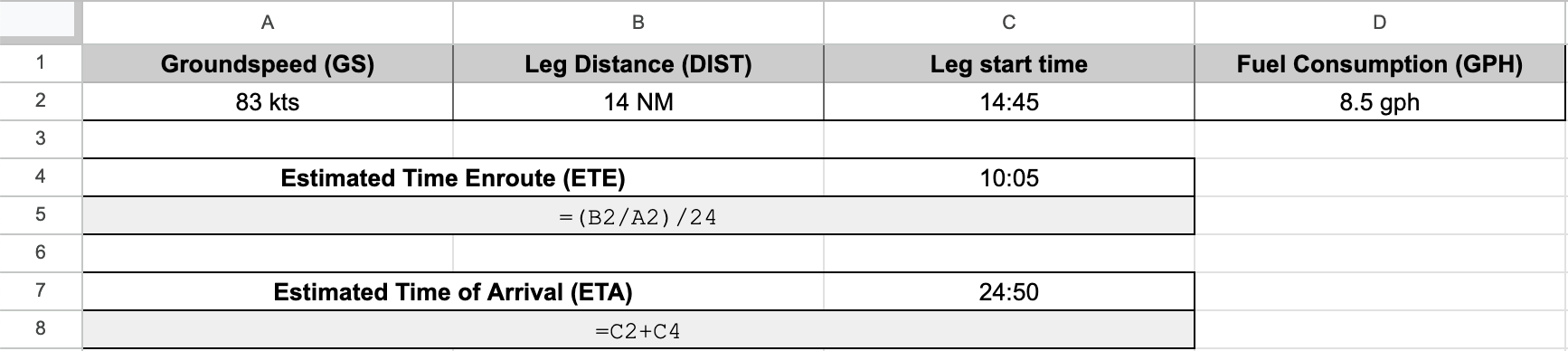
With the following cell assignment:

• Leg start time in cell C2
• The previously computed Estimated Time Enroute in cell C4

The following formula yields the estimated time of arrival:

=C2+C4

You can see an example below, and look at the second tab in the example worksheet here.

Leg fuel

With a known fuel consumption per hour figure, taken from our POH, it’s easy to derive the fuel required for the leg. Just remember that your Estimated Time Enroute is in days, so don’t forget to multiply that figure by 24 before you multiply it by the fuel consumption. With the following cell assignment:

• Fuel Consumption (GPH) in cell D2.
• The previously computed Estimated Time Enroute in cell C4.

The following formula yields the required leg fuel:

=C4*24*D2

You can see an example below, and look at the second tab in the example worksheet here.